So… Who Actually Runs the Model?

Another long story.

At this point, I had a model. I had explored quantization. I even had a DGX Spark sitting on my desk.

I thought I understood inference.

Then I kept seeing names like Ollama, llama.cpp, vLLM, and TensorRT-LLM everywhere.

People compared them. People said one was faster than another.

But nobody answered the question I actually had:

Who is really running the model?

A model sitting inside a GGUF or Safetensors file doesn’t generate a single token on its own.

Something has to:

• Load the model
• Tokenize the prompt
• Schedule GPU work
• Manage the KV cache
• Generate tokens
• Stream the response back

That “something” turned out to be the inference engine.

1. What Happens When I Enter a Prompt?

I started with a simple question:

What happens when I enter a prompt such as: “Explain supervised vs unsupervised learning in 3 sentences.”

The journey looks roughly like this:

Prompt Text
     │
     ▼
Tokenizer
     │
     ▼
Token IDs
     │
     ▼
Prefill Phase
     │
     ├── Process the input tokens
     ├── Perform the initial computation
     └── Build the KV cache
     │
     ▼
Decode Loop
     │
     ├── Predict one token at a time
     ├── Reuse the KV cache
     └── Append new KV values
     │
     ▼
Detokenizer
     │
     ▼
Streamed Answer

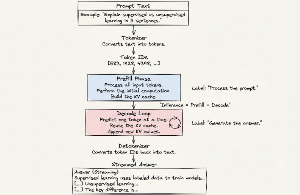
This was probably the first diagram that made inference click for me.

I had assumed inference was one continuous process. It isn’t. There are two very different phases: prefill and decode.

Prefill	Decode
Processes the input prompt	Generates one token at a time
Performs substantial computation	Repeatedly reads model weights and KV cache
Often makes better use of GPU compute	Is often more sensitive to memory bandwidth
Builds the KV cache	Extends and reuses the KV cache

The distinction was important.

Prefill is about processing the prompt. Decode is about generating the answer one token at a time.

2. So, What Actually Runs the Model?

The model itself is not “running.” The inference engine orchestrates the execution.

My first practical stop was llama.cpp.

I initially thought it was simply a tool for running .gguf models. But after looking at its structure, I realized it was an entire inference stack.

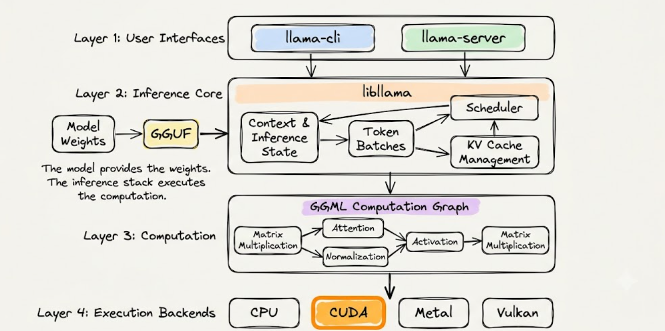
The llama-cli and llama-server provide user-facing interfaces, while libllama coordinates the inference process.

Inside the stack:

• The context and scheduler manage inference state, token batches, and KV-cache-related work.
• The GGML computation graph represents tensor operations.
• GGML backends determine where those operations run.
• The workload can use backends such as CPU, CUDA, Metal, or Vulkan.

In simple terms:

llama.cpp takes the model weights, prepares the computation, manages the inference state, and executes the workload on available hardware.

That became my first real example of what an inference engine actually does.

2.1 Where Does Ollama Fit?

Ollama presented a much simpler interface.

I could pull a model, run it, and interact with it through a familiar command:

ollama run llama3.1:8b

That simplicity is the main attraction.

Ollama provides a higher-level experience around local model execution, including:

• Model management
• Model packaging and distribution
• A local API
• Convenient commands
• Runtime configuration
• Integration with local applications

In many common GGUF-based workflows, Ollama uses llama.cpp-related execution components underneath. So I found it more useful to think of Ollama as a higher-level local model and runtime layer, rather than treating it as an entirely unrelated execution engine.

The distinction became important:

Ollama gives me convenience. llama.cpp gives me more direct visibility into execution.

3. Looking Beyond llama.cpp

After exploring llama.cpp, I looked at other runtimes that approach inference from different angles.

vLLM

vLLM is designed mainly for high-throughput model serving.

Its continuous batching and efficient KV-cache management make it interesting for APIs, agent workflows, and workloads where several requests share the same model.

TensorRT-LLM

TensorRT-LLM takes a more NVIDIA-focused approach.

It uses optimized kernels, graph-level optimizations, and hardware-specific execution paths to extract more performance from supported NVIDIA GPUs.

The difference became clearer to me:

• llama.cpp focuses on flexible local execution.
• vLLM focuses on serving efficiency and concurrent workloads.
• TensorRT-LLM focuses on optimized execution for NVIDIA hardware.

These are not simply steps in one pipeline. They are different approaches to the same problem:

How can we execute a model efficiently on available hardware?

4. GPU Mechanics: Where Does the Performance Come From?

Understanding inference engines was only one part of the story.

I then started wondering:

Why can two engines running the same model behave so differently?

The answer took me closer to how GPUs actually execute inference.

4.1 Arithmetic Intensity: Compute or Memory?

A GPU performs a huge number of mathematical operations, but it also needs to move data between memory and compute units.

This led me to arithmetic intensity — the relationship between the amount of computation performed and the amount of data moved.

In simple terms:

• High arithmetic intensity: More computation per byte of memory movement. The workload is often compute-bound.
• Low arithmetic intensity: More data movement compared with computation. The workload is often memory-bandwidth-bound.

This helped me understand the two main stages of inference:

• Prefill: Processes many input tokens together. It usually performs more computation and can make better use of the GPU’s compute units.
• Decode: Generates one token at a time while repeatedly reading model weights and the KV cache. It is often more sensitive to memory bandwidth.

So even when a GPU has powerful compute capability, generation may still be limited by how quickly data can move through memory.

4.2 Batching: Keeping the GPU Busy

The next concept was batching.

Instead of processing every request independently, an inference engine can process work from multiple requests together.

For example:

Request 1 → Token A
Request 2 → Token B
Request 3 → Token C

Processing these together can improve GPU utilization because the engine has more work available at the same time.

However, requests do not all have the same prompt length or generation length. Some finish quickly, while others continue generating.

This is where continuous batching becomes useful.

When one request finishes, the engine can introduce another request instead of waiting for the entire batch to complete.

4.3 KV-Cache Management: The Tetris Analogy

The KV cache made batching even more interesting.

I started imagining GPU memory as a Tetris board.

Every inference request is a different-shaped block:

• A short prompt needs a smaller KV cache.
• A long conversation needs a larger KV cache.
• A request generating many tokens keeps growing its KV cache.
• Different requests finish at different times.

With a simple allocation strategy, the engine may reserve large regions of memory for requests. As requests finish, the available space can become difficult to reuse efficiently.

The inference engine is essentially playing Tetris with memory.

More advanced approaches divide KV-cache memory into smaller blocks and reuse those blocks as requests arrive and finish. Combined with continuous batching, this allows the engine to keep the GPU busy while managing memory more flexibly.

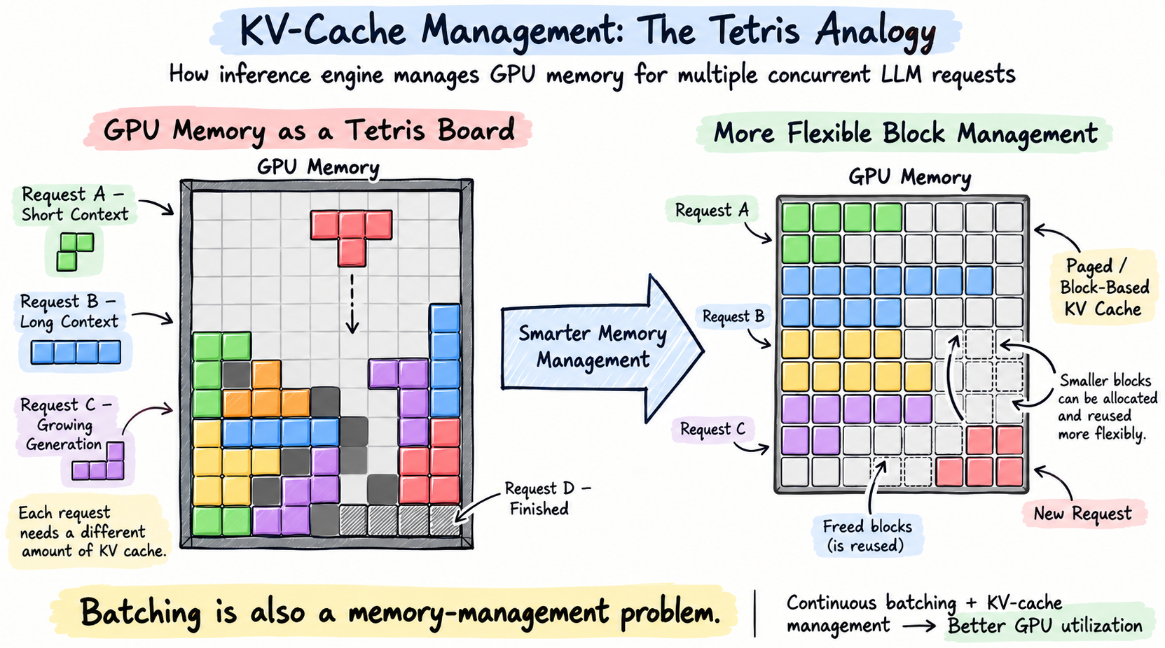
This was the point where batching stopped looking like just a performance trick.

Batching is also a memory-management problem.

And KV-cache management is one reason why different inference engines can behave very differently under concurrent workloads.

5. Moving From Concepts to an Experiment

At this point, I had learned enough theory to ask a more practical question:

Can I actually observe these differences on my own hardware?

Rather than trying to benchmark every model, context length, and runtime, I decided to keep the experiment small and controlled.

The goal wasn’t to declare one inference engine the universal winner. I wanted to understand how different runtimes behaved under the same workload, especially as concurrency increased.

I kept the following fixed:

• Same model family and model size
• Same hardware
• Same prompt
• Same output length
• Same temperature

I tested three runtimes using the model representations I had been exploring:

• Ollama / llama.cpp — Llama 3.1 8B, Q4_K_M
• vLLM — Llama 3.1 8B, FP8
• TensorRT-LLM — Llama 3.1 8B, NVFP4

This wasn’t a perfectly apples-to-apples benchmark because the model representations differed. I wasn’t trying to produce a universal ranking. I wanted to understand how these inference stacks behaved on my DGX Spark.

I used a fixed long-context prompt, generated up to 512 tokens, and tested two concurrency levels:

• N=1 — one request
• N=4 — four concurrent requests

5.1 Benchmark Results

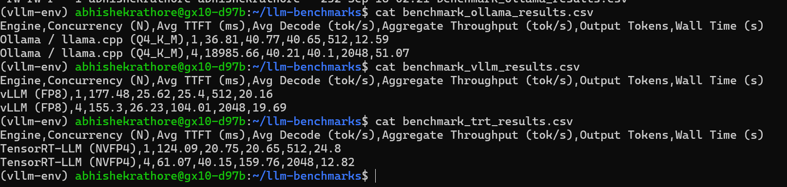
Inference Engine	Format	N	Avg TTFT	Avg Decode	Aggregate Throughput	Output Tokens	Wall Time
Ollama / llama.cpp	Q4_K_M	1	36.81 ms	40.77 tok/s	40.65 tok/s	512	12.59 s
Ollama / llama.cpp	Q4_K_M	4	18.99 s	40.21 tok/s	40.10 tok/s	2048	51.07 s
vLLM	FP8	1	177.48 ms	25.62 tok/s	25.40 tok/s	512	20.16 s
vLLM	FP8	4	155.30 ms	26.23 tok/s	104.01 tok/s	2048	19.69 s
TensorRT-LLM	NVFP4	1	124.09 ms	20.75 tok/s	20.65 tok/s	512	24.80 s
TensorRT-LLM	NVFP4	4	61.07 ms	40.15 tok/s	159.76 tok/s	2048	12.82 s

5.2 What the Numbers Showed Me

At N=1, Ollama had the highest decode rate in my setup.

But at N=4, the picture changed dramatically.

Ollama remained almost flat:

40.65 → 40.10 tok/s

vLLM increased from:

25.40 → 104.01 tok/s

TensorRT-LLM increased from:

20.65 → 159.76 tok/s

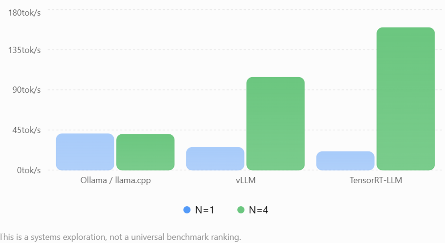The aggregate throughput scaling looked like this:

Runtime	N=1 → N=4
Ollama / llama.cpp	0.99×
vLLM	4.09×
TensorRT-LLM	7.74×

This was the moment the theory started making sense to me.

The fastest runtime for a single request isn’t necessarily the fastest runtime when multiple requests arrive.

The experiment wasn’t enough to explain exactly why. The runtimes used different execution strategies and model representations, so these results should not be treated as a universal ranking.

But they gave me something much more valuable:

I could finally see the concepts I had been reading about showing up as measurable behavior on my own machine.

And that sent me straight into the next rabbit hole:

Batching, scheduling, and KV-cache management.